Summary of Machine Learning and Artificial Intelligence Capabilities
Machine Learning (ML) is a field of Artificial Intelligence (AI) that enables computers to learn from data, without being explicitly programmed. Machine learning algorithms build models based on sample data, known as “training data”, in order to make predictions or decisions, rather than following rules written by humans. Machine learning is closely related to and often overlaps with computational statistics; a discipline that also focuses on prediction-making through the use of computers. Machine learning can be applied in a wide variety of domains, such as medical diagnosis, stock trading, robot control, manufacturing and more.
The process of machine learning consists of several steps: first, data is collected; then, a model is selected or created; finally, the model is trained on the collected data and then applied to new data. This process is often referred to as the “machine learning pipeline”. Problem formulation is the second step in this pipeline and it consists of selecting or creating a suitable model for the task at hand and determining how to represent the collected data so that it can be used by the selected model. In other words, problem formulation is the process of taking a real-world problem and translating it into a format that can be solved by a machine learning algorithm.
There are many different types of machine learning problems, such as classification, regression, prediction and so on. The choice of which type of problem to formulate depends on the nature of the task at hand and the type of data available. For example, if we want to build a system that can automatically detect fraudulent credit card transactions, we would formulate a classification problem. On the other hand, if our goal is to predict the sale price of houses given information about their size, location and age, we would formulate a regression problem. In general, it is best to start with a simple problem formulation and then move on to more complex ones if needed.
Some common examples of problem formulations in machine learning are:
– Classification: given an input data point (e.g., an image), predict its category label (e.g., dog vs cat).
– Regression: given an input data point (e.g., size and location of a house), predict a continuous output value (e.g., sale price).
– Prediction: given an input sequence (e.g., a series of past stock prices), predict the next value in the sequence (e.g., future stock price).
– Anomaly detection: given an input data point (e.g., transaction details), decide whether it is normal or anomalous (i.e., fraudulent).
– Recommendation: given information about users (e.g., age and gender) and items (e.g., books and movies), recommend items to users (e.g., suggest books for someone who likes romance novels).
– Optimization: given a set of constraints (e.g., budget) and objectives (e.g., maximize profit), find the best solution (e.g., product mix).
ML PRO without ADS on iOs [No Ads]
ML PRO without ADS on Windows [No Ads]
ML PRO For Web/Android on Amazon [No Ads]
The problem formulation phase of the ML Pipeline is critical, and it’s where everything begins. Typically, this phase is kicked off with a question of some kind. Examples of these kinds of questions include: Could cars really drive themselves? What additional product should we offer someone as they checkout? How much storage will clients need from a data center at a given time?
The problem formulation phase starts by seeing a problem and thinking “what question, if I could answer it, would provide the most value to my business?” If I knew the next product a customer was going to buy, is that most valuable? If I knew what was going to be popular over the holidays, is that most valuable? If I better understood who my customers are, is that most valuable?
However, some problems are not so obvious. When sales drop, new competitors emerge, or there’s a big change to a company/team/org, it can be easy to say, “I see the problem!” But sometimes the problem isn’t so clear. Consider self-driving cars. How many people think to themselves, “driving cars is a huge problem”? Probably not many. In fact, there isn’t a problem in the traditional sense of the word but there is an opportunity. Creating self-driving cars is a huge opportunity. That doesn’t mean there isn’t a problem or challenge connected to that opportunity. How do you design a self-driving system? What data would you look at to inform the decisions you make? Will people purchase self-driving cars?
Part of the problem formulation phase includes seeing where there are opportunities to use machine learning.
In the following practice examples, you are presented with four different business scenarios. For each scenario, consider the following questions:
The solutions given in this article are one of the many ways you can formulate a business problem.
In conclusion, problem formulation is an important step in the machine learning pipeline that should not be overlooked or underestimated. It can make or break a machine learning project; therefore, it is important to take care when formulating machine learning problems.”
Feature Engineering is the act of reshaping and curating existing data to make patters more apparent. This process makes the data easier for an ML model to understand. Using knowledge of the data, features are engineered and tuned to make ML algorithms work more efficiently.
For this problem, imagine a scenario where you are running a real estate brokerage and you want to predict the selling price of a house. Using a specific county dataset and simple information (like the location, total square footage, and number of bedrooms), let’s practice training a baseline model, conducting feature engineering, and tuning a model to make a prediction.
First, load the dataset and take a look at its basic properties.
# Load the dataset
import pandas as pd
import boto3
df = pd.read_csv(“xxxxx_data_2.csv”)
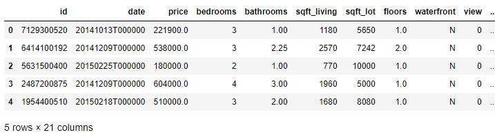
df.head()
Output:
This dataset has 21 columns:
id – Unique id numberdate – Date of the house saleprice – Price the house sold forbedrooms – Number of bedroomsbathrooms – Number of bathroomssqft_living – Number of square feet of the living spacesqft_lot – Number of square feet of the lotfloors – Number of floors in the housewaterfront – Whether the home is on the waterfrontview – Number of lot sides with a viewcondition – Condition of the housegrade – Classification by construction qualitysqft_above – Number of square feet above groundsqft_basement – Number of square feet below groundyr_built – Year builtyr_renovated – Year renovatedzipcode – ZIP codelat – Latitudelong – Longitudesqft_living15 – Number of square feet of living space in 2015 (can differ from sqft_living in the case of recent renovations)sqrt_lot15 – Nnumber of square feet of lot space in 2015 (can differ from sqft_lot in the case of recent renovations)This dataset is rich and provides a fantastic playground for the exploration of feature engineering. This exercise will focus on a small number of columns. If you are interested, you could return to this dataset later to practice feature engineering on the remaining columns.
Now, let’s train a baseline model.
People often look at square footage first when evaluating a home. We will do the same in the oflorur model and ask how well can the cost of the house be approximated based on this number alone. We will train a simple linear learner model (documentation). We will compare to this after finishing the feature engineering.
import sagemaker
import numpy as np
from sklearn.model_selection import train_test_split
import time
t1 = time.time()
# Split training, validation, and test
ys = np.array(df[‘price’]).astype(“float32”)
xs = np.array(df[‘sqft_living’]).astype(“float32”).reshape(-1,1)
np.random.seed(8675309)
train_features, test_features, train_labels, test_labels = train_test_split(xs, ys, test_size=0.2)
val_features, test_features, val_labels, test_labels = train_test_split(test_features, test_labels, test_size=0.5)
# Train model
linear_model = sagemaker.LinearLearner(role=sagemaker.get_execution_role(),
instance_count=1,
instance_type=’ml.m4.xlarge’,
predictor_type=’regressor’)
train_records = linear_model.record_set(train_features, train_labels, channel=’train’)
val_records = linear_model.record_set(val_features, val_labels, channel=’validation’)
test_records = linear_model.record_set(test_features, test_labels, channel=’test’)
linear_model.fit([train_records, val_records, test_records], logs=False)
sagemaker.analytics.TrainingJobAnalytics(linear_model._current_job_name, metric_names = [‘test:mse’, ‘test:absolute_loss’]).dataframe()
If you examine the quality metrics, you will see that the absolute loss is about $175,000.00. This tells us that the model is able to predict within an average of $175k of the true price. For a model based upon a single variable, this is not bad. Let’s try to do some feature engineering to improve on it.
Throughout the following work, we will constantly be adding to a dataframe called encoded. You will start by populating encoded with just the square footage you used previously.
encoded = df[[‘sqft_living’]].copy()
Let’s start by including some categorical variables, beginning with simple binary variables.
The dataset has the waterfront feature, which is a binary variable. We should change the encoding from 'Y' and 'N' to 1 and 0. This can be done using the map function (documentation) provided by Pandas. It expects either a function to apply to that column or a dictionary to look up the correct transformation.
Let’s write code to transform the waterfront variable into binary values. The skeleton has been provided below.
encoded[‘waterfront’] = df[‘waterfront’].map({‘Y’:1, ‘N’:0})
You can also encode many class categorical variables. Look at column condition, which gives a score of the quality of the house. Looking into the data source shows that the condition can be thought of as an ordinal categorical variable, so it makes sense to encode it with the order.
Using the same method as in question 1, encode the ordinal categorical variable condition into the numerical range of 1 through 5.
encoded[‘condition’] = df[‘condition’].map({‘Poor’:1, ‘Fair’:2, ‘Average’:3, ‘Good’:4, ‘Very Good’:5})
A slightly more complex categorical variable is ZIP code. If you have worked with geospatial data, you may know that the full ZIP code is often too fine-grained to use as a feature on its own. However, there are only 7070 unique ZIP codes in this dataset, so we may use them.
However, we do not want to use unencoded ZIP codes. There is no reason that a larger ZIP code should correspond to a higher or lower price, but it is likely that particular ZIP codes would. This is the perfect case to perform one-hot encoding. You can use the get_dummies function (documentation) from Pandas to do this.
Using the Pandas get_dummies function, add columns to one-hot encode the ZIP code and add it to the dataset.
encoded = pd.concat([encoded, pd.get_dummies(df[‘zipcode’])], axis=1)
In this way, you may freely encode whatever categorical variables you wish. Be aware that for categorical variables with many categories, something will need to be done to reduce the number of columns created.
One additional technique, which is simple but can be highly successful, involves turning the ZIP code into a single numerical column by creating a single feature that is the average price of a home in that ZIP code. This is called target encoding.
To do this, use groupby (documentation) and mean (documentation) to first group the rows of the DataFrame by ZIP code and then take the mean of each group. The resulting object can be mapped over the ZIP code column to encode the feature.
Complete the following code snippet to provide a target encoding for the ZIP code.
means = df.groupby(‘zipcode’)[‘price’].mean()
encoded[‘zip_mean’] = df[‘zipcode’].map(means)
Normally, you only either one-hot encode or target encode. For this exercise, leave both in. In practice, you should try both, see which one performs better on a validation set, and then use that method.
Take a look at the dataset. Print a summary of the encoded dataset using describe (documentation).
encoded.describe()
One column ranges from 290290 to 1354013540 (sqft_living), another column ranges from 11 to 55 (condition), 7171 columns are all either 00 or 11 (one-hot encoded ZIP code), and then the final column ranges from a few hundred thousand to a couple million (zip_mean).
In a linear model, these will not be on equal footing. The sqft_living column will be approximately 1300013000 times easier for the model to find a pattern in than the other columns. To solve this, you often want to scale features to a standardized range. In this case, you will scale sqft_living to lie within 00 and 11.
Fill in the code skeleton below to scale the column of the DataFrame to be between 00 and 11.
sqft_min = encoded[‘sqft_living’].min()
sqft_max = encoded[‘sqft_living’].max()
encoded[‘sqft_living’] = encoded[‘sqft_living’].map(lambda x : (x-sqft_min)/(sqft_max – sqft_min))
cond_min = encoded[‘condition’].min()
cond_max = encoded[‘condition’].max()
encoded[‘condition’] = encoded[‘condition’].map(lambda x : (x-cond_min)/(cond_max – cond_min))]
Predicting Credit Card Fraud Solution
Predicting Airplane Delays Solution
Data Processing for Machine Learning Example
Offering employees, coworkers, teammates, and students constructive feedback is a vital part of growth on…
Millennials should avoid delaying the inevitable and look into various retirement investment pathways. Here’s why…
For most people, a satisfactory career is essential for leading a happy life. However, ensuring…
The pipeline industry is more than pipework and construction, and we explore those details in…
SQL Interview Questions and Answers In the world of data-driven decision-making, SQL (Structured Query Language)…